Develop mathematical model of age of water and carbon
Contents
Concept
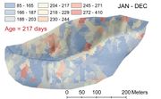
From the physical science perspective this research focuses on theoretical and experimental aspects of the isotopic “age” of water and carbon in lake-catchment systems. In this context, “age” is defined as the time since the water parcel and environmental tracer entered the system as precipitation. We note that each of our communities have developed an observing system for isotope ratios of carbon, oxygen and hydrogen but with very different science questions. In this research we will test a framework using models and data for defining a unified “isoscape” for the watershed-lake system, forming a richer and more collaborative shared research strategy. Our hypothesis is that the lake-catchment isoscape provides the experimental basis for predicting flow paths, residence times and the relative age of water in space and time, and that understanding these spatiotemporal patterns will provide a deeper understanding of fundamental biogeochemical processes including carbon and nitrogen cycling within the lake-catchment system. There is a wide literature on the use of residence time and relative age distribution of isotopes in environmental systems. Theories have been proposed using tracers for age modeling in ocean ventilation, atmospheric circulation, soil water, stream, groundwater flow, biophysics of vegetation photosynthesis as well as the circulation of blood. We begin this research with a simple model for the age of an environmental tracers in a ecohydrologic setting. Details of the approach can be found in Duffy (2010). The figure below is a simulation for the space-time distribution of isotopic age from the Shale Hills Critical Zone Observatory (Bhatt, 2012).
A useful analogy to understand the concept of “age” comes from population biology (Forester, 1959; Rotenberg, 1972). Consider a random population of individuals (species or particles) being born, dying and migrating. Given a long-term census of the population, the distribution of the size of the population through time and the distribution of ages of the population through time can be evaluated. Other moments may also be useful and can easily be determined from the census given enough data. The important concept to consider here is that there are actually two things we wish to evaluate in our long-term census: the number of individuals in our population through time, and the mean age of the population through time. For dissolved chemical species in water each component is characterized by physical time (clock time) and by the relative time or age since the species entered the system. The relative time for each component has it's own frame of reference particular to the dynamics of the flow system, the transport processes and the interaction with other components in the system.
In the broader context, our goal is to construct a predictive model for the fifth dimension of environmental tracers, the space-time-age distribution of the physical, chemical and biological pathways of the terrestrial environmental systems.
A Well-Mixed Lake
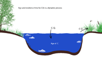
We begin with a simple lake or reservoir model for a single input and output as shown in Fig. 2. We define the isotopic “age” as the elapsed time since the particular tracer or isotope has entered the system as input. In other words the tracer is assumed to have zero age upon entering the lake. We note that in general, the tracer age is a statistical quantity that depends on the sources of tracer, the particular transport and flow processes, the biochemical interactions, as well as the boundaries and initial conditions of the physical system. Over the course of this project we will demonstrate the concept of “age” for a fully-coupled, spatially-distributed, lake-catchment system. In this basic example to follow we demonstrate how the age of the tracer is a simple extension of traditional ecohydrologic models.
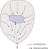
Figure 1 illustrates a simplified physical domain for this example. Typical observations for flow and tracer concentration would include sampling the lake inputs (precipitation, streamflow, groundwater, etc.), sampling the lake storage volume to determine the average values, and sampling the lake outputs (evapotranspiration, groundwater, surface outflow, etc.). From the introduction to this section recall that each tracer observation has two properties in this simple system: the physical or absolute time Failed to parse (Missing <code>texvc</code> executable. Please see math/README to configure.): t of the observation (e.g clock time), and the relative time since the sample entered the system, which is the age of the individual tracer Failed to parse (Missing <code>texvc</code> executable. Please see math/README to configure.): \tau . Assuming the tracer enters the system randomly, the joint distribution function describes the number of particles in the lake volume for time interval Failed to parse (Missing <code>texvc</code> executable. Please see math/README to configure.): dt and age interval Failed to parse (Missing <code>texvc</code> executable. Please see math/README to configure.): d \tau .In general, the functional form of c(t,Failed to parse (Missing <code>texvc</code> executable. Please see math/README to configure.): \tau ) is required to develop complete information on the joint age-time distribution for our experiment, and this might be accomplished by fitting a particular function to experimental data. However, it may be straight-forward to estimate the mass of our tracer in each sample volume, it is not generally feasible to determine the age of each sample. An alternative strategy is to relax the need for a colmplete description of the isotope population distribution and settle for a partial answer. That is, we assume c(t,Failed to parse (Missing <code>texvc</code> executable. Please see math/README to configure.): \tau ) exists but with an unknown functional form, and with certain constraints on the moments. The usual rules of probability apply and we can estimate the moments in t by integrating c(t,Failed to parse (Missing <code>texvc</code> executable. Please see math/README to configure.): \tau ) w/re to Failed to parse (Missing <code>texvc</code> executable. Please see math/README to configure.): \tau (see Delhez, 1999 or Duffy, 2010):
Failed to parse (Missing <code>texvc</code> executable. Please see math/README to configure.): \operatorname{\mu_n}(t) = \int_0^{\infty} \tau^{n}c(t,\tau)\,d\tau,\quad n=0,1,2...\quad (1)
The 0th and 1st moment of (1) are given by:
Failed to parse (Missing <code>texvc</code> executable. Please see math/README to configure.): \mathit{C}(t)=\operatorname{\mu_0}(t) = \int_0^{\infty} \tau^{0}c(t,\tau)\,d\tau,\quad n=0;\quad (2)
Failed to parse (Missing <code>texvc</code> executable. Please see math/README to configure.): \mathit{M}(t)=\operatorname{\mu_1}(t) =\int_0^{\infty} \tau^{1}c(t,\tau)\,d\tau,\quad n=1;\quad (3)
where we identify the 0th moment as the tracer concentration C(t) and M(t) the 1st moment of c(t,Failed to parse (Missing <code>texvc</code> executable. Please see math/README to configure.): \tau ). The key to our analysis is that the ratio of the 1st to 0th moment is the classical definition of the mean age of the system :
Failed to parse (Missing <code>texvc</code> executable. Please see math/README to configure.): \mathit{Age}= {\alpha}(t) = \frac{\mu_1}{\mu_0} \ =\frac{\mathit{M}(t)}{\mathit{C}(t)}\, \quad (4)
At this point we have defined the tracer as a dynamic variable that depends on the duration that the observation has spent in the lake, and the physical time describing the evolution of all tracer particles in the system. Equations (1-3) define the moment relations for our experiment, and the next step is to develop a physical model for the system.
For a single input and single output, we take the volumetric inflow rate to be Failed to parse (Missing <code>texvc</code> executable. Please see math/README to configure.): Qi [L^3/T]) , the outflow as Failed to parse (Missing <code>texvc</code> executable. Please see math/README to configure.): Q [L^3/T] , and for simplicity the flow is initially assumed to be at steady-state (Failed to parse (Missing <code>texvc</code> executable. Please see math/README to configure.): Qi =Q ). The input tracer Ci can be isotopes of water (Failed to parse (Missing <code>texvc</code> executable. Please see math/README to configure.): \delta^{18} O or Failed to parse (Missing <code>texvc</code> executable. Please see math/README to configure.): \delta^{2} H ), carbon or other solutes. As was the case in the population example given earlier, we expect the mass balance for our system to be conserved w/re to both time and age, and this is represented in the model as:
Failed to parse (Missing <code>texvc</code> executable. Please see math/README to configure.): \frac{\partial c}{\partial t}+\frac{\partial c}{\partial \tau}=\Gamma_c-\mathit{L}(c),\quad (5)
where the left hand side is the total derivative for time and age of the isotope, and the right hand side represents tracer inputs, transformations and outputs. Integrating (4) w/re to as in (1), and applying the moment equations (2) yields the following dynamical system for the first 2 moments {n=0,1}:
Failed to parse (Missing <code>texvc</code> executable. Please see math/README to configure.): \frac{\partial C}{\partial t}=k\left ( \mathit{C_i} - \mathit{C} \right )
Failed to parse (Missing <code>texvc</code> executable. Please see math/README to configure.): \frac{\partial M}{\partial t}=\left ( \mathit{C}- k\mathit{M} \right )\qquad (6)
Failed to parse (Missing <code>texvc</code> executable. Please see math/README to configure.): \mathit{Age}= {\alpha}(t) =\frac{\mathit{M}(t)}{\mathit{C}(t)},\quad
Failed to parse (Missing <code>texvc</code> executable. Please see math/README to configure.): {\alpha}(\infty) =\frac{V}{Q} \ =\frac{\mathit{M}(\infty)}{\mathit{C}(\infty)}\,
where C(t) is tracer concentration, M(t) is the 1st moment, and their ratio is the the age Failed to parse (Missing <code>texvc</code> executable. Please see math/README to configure.): \alpha (t) and Failed to parse (Missing <code>texvc</code> executable. Please see math/README to configure.): \alpha (\infty) is the steady-state age of the lake, with input Ci . It should be noted that for a well-mixed reservoir, the steady-state age of the tracer is identical to the mean age of the tracer leaving the system (e.g. the steady-state residence time). Equation (6) shows that the age and residence time are actually dynamic quantities, with a constant asymptotic- or long-term average value. The asymptotic value is the traditional steady-state residence time.
The system (6) admits a closed form solution for steady flow conditions (Qi =Q), with constant input (Ci) and uniform initial conditions (C(0)=C0):
Failed to parse (Missing <code>texvc</code> executable. Please see math/README to configure.): \mathit{C}(t)=e^{-kt}\left ( \ \mathit{C_0}- \mathit{C_i}+ \mathit{C_i}e^{kt}\right )\,Failed to parse (Missing <code>texvc</code> executable. Please see math/README to configure.): \mathit{M}(t)=\frac{e^{-kt}}{k}\left ( \ \mathit{C_i}e^{kt}- \mathit{C_i}+ \mathit{C_0}kt-\mathit{C_i}kt\right )\, \quad (7)
Failed to parse (Missing <code>texvc</code> executable. Please see math/README to configure.): \alpha(t)=\frac{\left ( \ \mathit{C_i}e^{kt}- \mathit{C_i}+ \mathit{C_0}kt- \mathit{C_i}kt\right )}{k\left ( \mathit{C_0}- \mathit{C_i}+ \mathit{C_i}e^{kt}\right )}\,
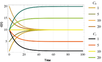
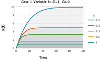
For purpose of discussion, Fig. 3 illustrates the tracer concentration solution trajectories for a range of initial conditions and inputs. Figure 4 illustrates the solution for the mean age of the tracer in the lake. It is important to realize that tracer age in the dynamical model is a relative quantity that also depends on the initial conditions and asymptotic “age” of the system at steady-state. In this case we assume the initial tracer age in the lake is α(t)=0 and the inputs Ci are zero age as they enter the lake (e.g. a birth in the population context). Of course other initial and input conditions are possible. Note that as
Failed to parse (Missing <code>texvc</code> executable. Please see math/README to configure.): Q\Rightarrow 0\quad and Failed to parse (Missing <code>texvc</code> executable. Please see math/README to configure.): C_i\Rightarrow 0\quad , the system simply ages in clock time or the solution (7) is Failed to parse (Missing <code>texvc</code> executable. Please see math/README to configure.): \alpha= t .
Case 1: Variable V/Q
The solutions for variable in Fig. 4 shows the impact of varying the rate constant k (or steady-state age α( )=k-1) when the input concentration exceeds the initial condition, Ci. ≥ C0. The dynamic age of the tracer evolves from zero age to the asymptotic steady-state value. We see that the average age of the tracer in the lake and, by the well-mixed assumption, the age of the tracer in the outflow, will reach a constant age.
Case 2: Variable Initial Condition Co
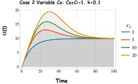
The solutions for in Fig. 5 demonstrates that age calculations in models must be thought of as “relative age”, or the age since the start of the experiment. The initial condition C0 in Fig. 5 is varied while holding the input value at Ci=1. Note that when C0 > Ci, the early time age (t<V/Q) grows until the older water is displaced. The greater the concentration difference (C0 - Ci), the greater the effect on early time age. At late time in the event, the age solution gradually approaches the asymptotic age Failed to parse (Missing <code>texvc</code> executable. Please see math/README to configure.): \alpha (\infty) .
In the catchment hydrology literature there has been a long- standing discussion about how to interpret the age of runoff. Typically, experiments find that old water or pre-event water chemical signatures dominate the runoff response during and after rainfall events (e.g. the runoff event concentration is much different than the precipitation concentration. It would seem that this simple experiment (case 2) explains why field observations of old water following an input event can be explained as a simple function of two conditions: the difference between the initial and input concentrations (C0 - Ci), and the steady-state age V/Q of the system.
Case 3: Variable Input Ci
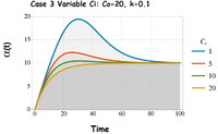
In case 3 (Fig. 6) the input for the tracer was varied, for a constant initial concentration (C0 =20). Again note that the early time age is depends on the difference (C0 - Ci) and the steady-state age is V/Q=10 years.
Case 4: Variable Initial Age α(0)
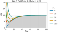
In cases 1-3, the initial condition for tracer age in the lake was assumed to be Failed to parse (Missing <code>texvc</code> executable. Please see math/README to configure.): \alpha (0)=0 . In Case 4 we examine the effect of varying the initial age of the lake water and the solutions are given in Fig. 7. In systems where the initial age is old relative to the characteristic time of our system, the initially old water evolves to the new steady-state age in approximately 3 characteristic time scales, t~3V/Q. This example could be applied to the problem of assessing the impact of management practices, where contaminant inputs have been reduced and the time it takes to see the impacts on the lake or lake outflow is of interest. Performance assessment from reduced nutrient loading from agricultural runoff, or reduced atmospheric pollutants from the energy production and atmospheric contaminants, could apply a dynamic ageing model to assess the time it might take to measure the value of management practices and time to ecosystem recovery.
Reactions, Sources and Sinks
The case of solute interactions is examined next for a 2-component reactive system in series under unsteady flow conditions. Consider the transient 2-component model where the first component is a source term for the 2nd and the 2nd component is subject to first-order loss.Failed to parse (Missing <code>texvc</code> executable. Please see math/README to configure.): \frac{\partial \mathit{V}}{\partial t}= \mathit{Q_i} - \mathit{Q}
Failed to parse (Missing <code>texvc</code> executable. Please see math/README to configure.): \frac{\partial \mathit{V C_1}}{\partial t}= \mathit{Q_i}\mathit{C_{1i}} -\mathit{k_1 VC_1} - \mathit{QC_1}
Failed to parse (Missing <code>texvc</code> executable. Please see math/README to configure.): \frac{\partial \mathit{V C_2}}{\partial t}= \mathit{Q_i}\mathit{C_{2i}} +\mathit{k_1 VC_1} - \mathit{k_2 VC_2} - \mathit{QC_2}
where Failed to parse (Missing <code>texvc</code> executable. Please see math/README to configure.): Q_i
is the net lake input flux, Failed to parse (Missing <code>texvc</code> executable. Please see math/README to configure.): Q_{s}
is the lake input flux from streams, Failed to parse (Missing <code>texvc</code> executable. Please see math/README to configure.): Q
is lake outflow, Failed to parse (Missing <code>texvc</code> executable. Please see math/README to configure.): V
is the lake volume, Failed to parse (Missing <code>texvc</code> executable. Please see math/README to configure.): C_{1i}
and Failed to parse (Missing <code>texvc</code> executable. Please see math/README to configure.): C_{2i}
are the lake inputs, Failed to parse (Missing <code>texvc</code> executable. Please see math/README to configure.): k_1, k_2
are first order reaction rates and the subscripts refers to each reactive tracer. The observed net inputs are given by:
Failed to parse (Missing <code>texvc</code> executable. Please see math/README to configure.): \mathit{Q_i}= Q_{s}+A_s P-A_s ET
Failed to parse (Missing <code>texvc</code> executable. Please see math/README to configure.): \mathit{C_{ji}}= \left(\frac{Q_{in}}{ \mathit{Q_i}} \mathit{C_{in}}+ \frac{\mathit{A_s P}}{ \mathit{Q_i}} \mathit{C_p}- \frac{\mathit{A_s ET}}{ \mathit{Q_i}} \mathit{C_{ET}}\right )_j, j=1,2
The zero-moment of tracer concentration equations are rearranged to form a simplified dynamical system:
Failed to parse (Missing <code>texvc</code> executable. Please see math/README to configure.): V \frac{\partial \mathit{C_1}}{\partial t}= Q_i\left (\mathit{C_{1i}} - \mathit{C_1} \right )-\mathit{k_1 VC_1}
Failed to parse (Missing <code>texvc</code> executable. Please see math/README to configure.): V \frac{\partial \mathit{C_2}}{\partial t}= Q_i\left (\mathit{C_{2i}} - \mathit{C_2} \right )+ \mathit{k_1 VC_1} - \mathit{k_2 VC_2}
The first moment equations for the 2-component system are given by:
Failed to parse (Missing <code>texvc</code> executable. Please see math/README to configure.): V \frac{\partial \mathit{M_1}}{\partial t}= \mathit{VC_1}- \mathit{Q_i M_1} - \mathit{k_1 VM_1}
Failed to parse (Missing <code>texvc</code> executable. Please see math/README to configure.): V \frac{\partial \mathit{M_2}}{\partial t} =\mathit{VC_2} -\mathit{Q_i M_2} + \mathit{k_1 VM_1}-\mathit{k_2 VM_2}
and the ratio of the first moment to the zeroth moment, or Age for the surface and deep layer are:
Failed to parse (Missing <code>texvc</code> executable. Please see math/README to configure.): \mathit{Age_1}= {\alpha_1}(t) =\frac{\mathit{M_1}(t)}{\mathit{C_1}(t)},\quad
Failed to parse (Missing <code>texvc</code> executable. Please see math/README to configure.): \mathit{Age_2}= {\alpha_2}(t) =\frac{\mathit{M_2}(t)}{\mathit{C_2}(t)},\quad
To summarize, estimating the age for this 2 component serial reactive system requires the solution of 4 equations: Failed to parse (Missing <code>texvc</code> executable. Please see math/README to configure.): C_1, C_2, M_1, M_2 , and the ratios Failed to parse (Missing <code>texvc</code> executable. Please see math/README to configure.): M_1/C_1, M_2/C_2 provide the age of each component. Note that this formulation shows that the age of each tracer depends on transient flow as well as tracer concentration.
The sequential model can be generalized for n reactions, Failed to parse (Missing <code>texvc</code> executable. Please see math/README to configure.): \mathit{j=1,2,3,..,n}
Failed to parse (Missing <code>texvc</code> executable. Please see math/README to configure.): V \frac{\partial \mathit{C_1}}{\partial t}= Q_i\left (\mathit{C_{1i}} - \mathit{C_1} \right )-\mathit{k_1 VC_1}
Failed to parse (Missing <code>texvc</code> executable. Please see math/README to configure.): V \frac{\partial \mathit{C_j}}{\partial t}= Q_i\left (\mathit{C_{ji}} - \mathit{C_j} \right )-\mathit{k_j VC_j}+\mathit{k_{j-1} VC_{j-1}}
and
Failed to parse (Missing <code>texvc</code> executable. Please see math/README to configure.): V \frac{\partial \mathit{M_1}}{\partial t}= \mathit{VC_1}- \mathit{Q_i M_1} - \mathit{k_1 VM_1}
Failed to parse (Missing <code>texvc</code> executable. Please see math/README to configure.): V \frac{\partial \mathit{M_j}}{\partial t}= \mathit{VC_{j}} - \mathit{Q_i M_j} -\mathit{k_j MA_j}+\mathit{k_{j-1} VM_{j-1}}
Well-Mixed Tracer and Transient Flow
We can extend the lake model to include transient flow. Following the same strategy as before the equations for flow and concentration have the form:Failed to parse (Missing <code>texvc</code> executable. Please see math/README to configure.): \frac{\partial \mathit{V}}{\partial t}= \mathit{Q_i} - \mathit{Q}
Failed to parse (Missing <code>texvc</code> executable. Please see math/README to configure.): \frac{\partial \left ( \mathit{VC}\right )}{\partial t}= \mathit{Q_i}\mathit{C_i} - \mathit{Q}\mathit{C}
where Failed to parse (Missing <code>texvc</code> executable. Please see math/README to configure.): Q_i is the lake input flux, Failed to parse (Missing <code>texvc</code> executable. Please see math/README to configure.): Q is lake outflow. Note that it is straight forward to include multiple input loadings Failed to parse (Missing <code>texvc</code> executable. Please see math/README to configure.): Q_i C_i, i=1,2,...n\quad . Expanding the 2nd equation and after some manipulation we arrive at our dynamical system for transient flow, tracer concentration and age for the lake assuming time variable storage-outflow:
Failed to parse (Missing <code>texvc</code> executable. Please see math/README to configure.): \frac{\partial \mathit{V}}{\partial t}= \mathit{Q_i} - \mathit{Q}
Failed to parse (Missing <code>texvc</code> executable. Please see math/README to configure.): \frac{\partial \mathit{C}}{\partial t}= \frac {1}{\tau_c} \left (\mathit{C_i} - \mathit{C} \right )
Failed to parse (Missing <code>texvc</code> executable. Please see math/README to configure.): \frac{\partial A}{\partial t}=\mathit{C}- \frac {1}{\tau_c}\mathit{A} \qquad
Failed to parse (Missing <code>texvc</code> executable. Please see math/README to configure.): \mathit{Age}= {\alpha}(t) =\frac{\mathit{A}(t)}{\mathit{C}(t)},\quad
Failed to parse (Missing <code>texvc</code> executable. Please see math/README to configure.): {\tau_c}(t) =\frac{V(t)}{Q_i(t)}
where V(t) is the time variable lake volume, C(t) is concentration and A(t) is 1st moment. The characteristic time in this case is not constant Failed to parse (Missing <code>texvc</code> executable. Please see math/README to configure.): {\tau_c}(t) and the equations are nonlinear which will require numerical solutions.
Two-Zone Lake Model with Incomplete Mixing
Next we develop a two-zone model with incomplete vertical exchange between the surface layer and a deeper stagnant layer. Failed to parse (Missing <code>texvc</code> executable. Please see math/README to configure.): V(t)= V_1 +V_2 is the total lake volume.Failed to parse (Missing <code>texvc</code> executable. Please see math/README to configure.): C_1 and Failed to parse (Missing <code>texvc</code> executable. Please see math/README to configure.): C_2 are the concentrations for each layer and the layers exchange mass by diffusion, while advection occurs only in the surface layer. The equations for flow and concentration have the form:Failed to parse (Missing <code>texvc</code> executable. Please see math/README to configure.): \frac{\partial \mathit{V_1}}{\partial t}= \mathit{Q_i} - \mathit{Q}
Failed to parse (Missing <code>texvc</code> executable. Please see math/README to configure.): \frac{\partial \mathit{V_1 C_1}}{\partial t}= \mathit{Q_i}\mathit{C_i} - \mathit{Q}\mathit{C} +E'\left ( C_2 -C_1\right )
Failed to parse (Missing <code>texvc</code> executable. Please see math/README to configure.): \frac{\partial \mathit{V_2 C_2}}{\partial t}= -E'\left ( C_2 -C_1\right )
where Failed to parse (Missing <code>texvc</code> executable. Please see math/README to configure.): Q_i is the net lake input flux, Failed to parse (Missing <code>texvc</code> executable. Please see math/README to configure.): Q is lake outflow, Failed to parse (Missing <code>texvc</code> executable. Please see math/README to configure.): V_1 and Failed to parse (Missing <code>texvc</code> executable. Please see math/README to configure.): V_2 are the volumes of the surface and deep layers and Failed to parse (Missing <code>texvc</code> executable. Please see math/README to configure.): E'=DA_s/l is a bulk diffusion coefficient where Failed to parse (Missing <code>texvc</code> executable. Please see math/README to configure.): D is molecular diffusion and Failed to parse (Missing <code>texvc</code> executable. Please see math/README to configure.): l is the length scale. In this case we assume the system has multiple observed inputs:
Failed to parse (Missing <code>texvc</code> executable. Please see math/README to configure.): \mathit{Q_i}= Q_{in}+A_s P+A_s ET
Failed to parse (Missing <code>texvc</code> executable. Please see math/README to configure.): \mathit{C_{i}}= \frac{Q_{in}}{ \mathit{Q_i}} \mathit{C_{in}}+ \frac{\mathit{A_s P}}{ \mathit{Q_i}} \mathit{C_p}+ \frac{\mathit{A_s ET}}{ \mathit{Q_i}} \mathit{C_{ET}}
where Failed to parse (Missing <code>texvc</code> executable. Please see math/README to configure.): \mathit{Q_{in}C_{in}}
is the input mass flow rate, Failed to parse (Missing <code>texvc</code> executable. Please see math/README to configure.): \mathit{P C_p}
is the precipitation loading rate, Failed to parse (Missing <code>texvc</code> executable. Please see math/README to configure.): \mathit{ET C_{ET}}
is evapotranspiration mass flux and Failed to parse (Missing <code>texvc</code> executable. Please see math/README to configure.): A_s
is the area of the lake or the surface area between Failed to parse (Missing <code>texvc</code> executable. Please see math/README to configure.): V_1
and Failed to parse (Missing <code>texvc</code> executable. Please see math/README to configure.): V_2
.
As before the equations are rearranged to form the simplified form of the dynamical system:
Failed to parse (Missing <code>texvc</code> executable. Please see math/README to configure.): V_1 \frac{\partial \mathit{C_1}}{\partial t}= Q_i\left (\mathit{C_i} - \mathit{C_1} \right )+E'\left (\mathit{C_2} - \mathit{C_1} \right )
Failed to parse (Missing <code>texvc</code> executable. Please see math/README to configure.): V_2 \frac{\partial \mathit{C_2}}{\partial t}= -E'\left (\mathit{C_2} - \mathit{C_1} \right )
The first moment equations are given by:
Failed to parse (Missing <code>texvc</code> executable. Please see math/README to configure.): V_1 \frac{\partial \mathit{A_1}}{\partial t}= \mathit{V_1 C_1}- \mathit{Q_i A_1} +E'\left (\mathit{A_2} - \mathit{A_1} \right )
Failed to parse (Missing <code>texvc</code> executable. Please see math/README to configure.): V_2 \frac{\partial \mathit{A_2}}{\partial t}=\mathit{V_2 C_2} -E'\left (\mathit{A_2} - \mathit{A_1} \right )
The ratio of the first moment to the zeroth moment is the Age for the surface and deep layer.
Failed to parse (Missing <code>texvc</code> executable. Please see math/README to configure.): \mathit{Age_1}= {\alpha_1}(t) =\frac{\mathit{A_1}(t)}{\mathit{C_1}(t)},\quad
Failed to parse (Missing <code>texvc</code> executable. Please see math/README to configure.): \mathit{Age_2}= {\alpha_2}(t) =\frac{\mathit{A_2}(t)}{\mathit{C_2}(t)},\quad
To summarize, estimating the ages for this 2 component system requires the solution of 4 equations: Failed to parse (Missing <code>texvc</code> executable. Please see math/README to configure.): C_1, C_2, A_1, A_2 , and ratios Failed to parse (Missing <code>texvc</code> executable. Please see math/README to configure.): A_1/C_1, A_2/C_2 are calculated to give the ages for the surface and deep layer respectively. Note that this formulation shows that the evolution of tracer age depends on both flow and tracer dynamics.
Lake-Catchment Dynamical System
Next we examine the coupled dynamics for a lake-catchment system where groundwater inputs/ouput to/from the lake are unknown and where surface water inputs and outputs to the lake are observed.Failed to parse (Missing <code>texvc</code> executable. Please see math/README to configure.): \frac{\partial \mathit{V_1}}{\partial t}= \mathit{Q_{1i}} - \mathit{Q_1}+\mathit{Q_{12}}
Failed to parse (Missing <code>texvc</code> executable. Please see math/README to configure.): \frac{\partial \mathit{V_2}}{\partial t}= \mathit{Q_{2i}} - \mathit{Q_2}-\mathit{Q_{12}}
Failed to parse (Missing <code>texvc</code> executable. Please see math/README to configure.): \frac{\partial \mathit{V_1 C_1}}{\partial t}= \mathit{Q_{1i}}\mathit{C_{1i}} -\mathit{Q_1 C_1} + \mathit{Q_{12}C_{12}}
Failed to parse (Missing <code>texvc</code> executable. Please see math/README to configure.): \frac{\partial \mathit{V_2 C_2}}{\partial t}= \mathit{Q_{2i}}\mathit{C_{2i}} -\mathit{Q_2 C_2} - \mathit{Q_{12}C_{12}}
where Failed to parse (Missing <code>texvc</code> executable. Please see math/README to configure.): Q_{ji}
(Failed to parse (Missing <code>texvc</code> executable. Please see math/README to configure.): j=1,2
) is the net input flux to the lake (Failed to parse (Missing <code>texvc</code> executable. Please see math/README to configure.): j=1
) and catchment (Failed to parse (Missing <code>texvc</code> executable. Please see math/README to configure.): j=2
) respectively, Failed to parse (Missing <code>texvc</code> executable. Please see math/README to configure.): i
indicates input, Failed to parse (Missing <code>texvc</code> executable. Please see math/README to configure.): Q_1
is lake outflow, Failed to parse (Missing <code>texvc</code> executable. Please see math/README to configure.): Q_2
is the catchment outflow to the stream, Failed to parse (Missing <code>texvc</code> executable. Please see math/README to configure.): V_1
is the lake storage volume, Failed to parse (Missing <code>texvc</code> executable. Please see math/README to configure.): V_2
is the catchment storage volume, Failed to parse (Missing <code>texvc</code> executable. Please see math/README to configure.): C_{1i}
and Failed to parse (Missing <code>texvc</code> executable. Please see math/README to configure.): C_{2i}
are the lake and catchment isotopic inputs. The multiple observed inputs are given by:
Failed to parse (Missing <code>texvc</code> executable. Please see math/README to configure.): \mathit{Q_{ji}}= \left (\mathit{A_j P}-\mathit{A_j ET}\right ), j=1,2
Failed to parse (Missing <code>texvc</code> executable. Please see math/README to configure.): \mathit{C_{ji}}= \left (\frac{\mathit{A_j P}}{ \mathit{Q_{ji}}} \mathit{C_p}- \frac{\mathit{A_j ET}}{ \mathit{Q_{ji}}} \mathit{C_{ET}}\right ), j=1,2
The zero-moment or tracer concentration equations can be rearranged to form a simplified dynamical system:
Failed to parse (Missing <code>texvc</code> executable. Please see math/README to configure.): V_1 \frac{\partial \mathit{C_1}}{\partial t}= Q_{1i}\left (\mathit{C_{1i}} - \mathit{C_1} \right )+Q_{12}\left (\mathit{C_{12}} - \mathit{C_1} \right )
Failed to parse (Missing <code>texvc</code> executable. Please see math/README to configure.): V_2 \frac{\partial \mathit{C_2}}{\partial t}= Q_{2i}\left (\mathit{C_{2i}} - \mathit{C_2} \right )-Q_{12}\left (\mathit{C_{12}} - \mathit{C_2} \right )
Note that Failed to parse (Missing <code>texvc</code> executable. Please see math/README to configure.): C_{12} depends on the direction of flow or the sign of Failed to parse (Missing <code>texvc</code> executable. Please see math/README to configure.): \pm Q_{12} .
Failed to parse (Missing <code>texvc</code> executable. Please see math/README to configure.): C_{12} = \begin{cases} C_1 & Q_{12} \le 0 \\ C_2 & \mbox{otherwise} \end{cases}
The first moment equations for the lake-catchment system are given by:
Failed to parse (Missing <code>texvc</code> executable. Please see math/README to configure.): V_1 \frac{\partial \mathit{M_1}}{\partial t}= \mathit{V_1 C_1}- \mathit{Q_{1i} M_1} + Q_{12}\left (\mathit{M_{12}} - \mathit{M_1} \right )
Failed to parse (Missing <code>texvc</code> executable. Please see math/README to configure.): V_2 \frac{\partial \mathit{M_2}}{\partial t} =\mathit{V_2 C_2} -\mathit{Q_{2i} M_2} -Q_{12}\left (\mathit{M_{12}} - \mathit{M_2} \right )
where again Failed to parse (Missing <code>texvc</code> executable. Please see math/README to configure.): M_{12} depends on the direction of flow or the sign of Failed to parse (Missing <code>texvc</code> executable. Please see math/README to configure.): \pm Q_{12} .
Failed to parse (Missing <code>texvc</code> executable. Please see math/README to configure.): M_{12} = \begin{cases} M_1 & Q_{12} \le 0 \\ M_2 & \mbox{otherwise} \end{cases}
and the ratio of the first moment to the zeroth moment, or Age for the surface and deep layer are:
Failed to parse (Missing <code>texvc</code> executable. Please see math/README to configure.): \mathit{Age_1}= {\alpha_1}(t) =\frac{\mathit{M_1}(t)}{\mathit{C_1}(t)},\quad
Failed to parse (Missing <code>texvc</code> executable. Please see math/README to configure.): \mathit{Age_2}= {\alpha_2}(t) =\frac{\mathit{M_2}(t)}{\mathit{C_2}(t)},\quad
To summarize, estimating the age for this lake-catchment system requires the solution of 4 equations: Failed to parse (Missing <code>texvc</code> executable. Please see math/README to configure.): C_1, C_2, A_1, A_2 , and the ratios Failed to parse (Missing <code>texvc</code> executable. Please see math/README to configure.): A_1/C_1, A_2/C_2 provide the age of each component. Note that this formulation shows that the age of each tracer depends on transient flow as well as tracer concentration.
